The Central Processing Unit (CPU) is the brain of a computer, and for IT professionals, assessing CPU stress is foundational knowledge. However, this task may not be as simple as you think. This is a 4-part article series aim to guide you in evaluating CPU stress.
Part 1: Single-Core CPU Utilization: Demystifies why processes have to wait even when CPU utilization appears low.
Part 2: Multi-Core CPU Utilization: Explores how multiple cores within a CPU complicate the assessment of CPU utilization.
Part 3: CPU Run Queue Size: A more accurate metric for evaluating CPU stress
Part 4: CPU Load: A numerical measure of CPU stress, it differs slightly between Linux and Unix.
Single-Core CPU Utilization
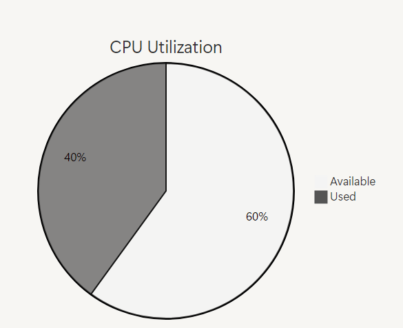
If CPU utilization is reported as 40%, you might assume that the 40% of CPU resources are busy and 60% remain available. If so, you are all wet. Unlike memory or disk space, CPU utilization isn’t a simple “used versus available” metric.
To fully understand CPU utilization, we need some background knowledge of processes and how the CPU operates. The basic execution unit of a CPU is cycle, the clock speed of CPU measures the number of cycles it executes per second, and is typically measured in GHz (gigahertz). For instance, a CPU with a clock speed of 3.2 GHz executes 3.2 billion cycles per second.
During each clock cycle, a CPU is either busy or idle—there’s no in-between. Within a single cycle, utilization is effectively 100% (busy) or 0% (idle); partial utilization doesn’t exist at this granularity. You can partially verify this using the Linux command mpstat -P ALL 1, which reports CPU utilization per core every second. The output often shows utilization pegged at 100% or 0%, reflecting the binary nature of cycle-level activity. However, since the smallest time interval for mpstat is one second, it aggregates many cycles, masking finer details. If we could measure at a shorter interval, the results would more accurately reflect this all-or-nothing behavior.
CPU utilization, as reported by the operating system, is a single statistical representation of how much the CPU was busy over a given interval. This is calculated as the number of busy cycles divided by the total number of cycles available in the interval.
Here is a ten-cycle interval where CPU utilization is 40%:
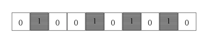
In this example, 4 cycles are busy, resulting in 40% CPU utilization over the ten-cycle interval. This metric helps in understanding how efficiently the CPU is being used during a specific timeframe.
In this scenario, runnable processes have a 40% chance of having to wait to use the CPU. These waiting processes form a queue known as the run queue. The longer the run queue, the more processes wait, increasing their time spent waiting. This debunks the common misconception that processes only wait when CPU utilization hits 100%. In reality, processes can experience wait times even at lower utilization levels due to the probabilistic nature of CPU scheduling.
The following table, the CPU Utilization Breakdown Table, illustrates how different utilization percentages affect scheduling probabilities:
| CPU Utilization | Chance of Running Immediately | Chance of Waiting |
|---|---|---|
| 50% | 1 in 2 (50%) | 1 in 2 (50%) |
| 66% | 1 in 3 (33.3%) | 2 in 3 (66.7%) |
| 80% | 1 in 5 (20%) | 4 in 5 (80%) |
| 90% | 1 in 10 (10%) | 9 in 10 (90%) |
- 50% Utilized: The process has a 50/50 chance of being scheduled immediately, meaning there is a 1 in 2 chance of running or waiting.
- 66% Utilized: There’s a 1 in 3 chance of running right away and a 2 in 3 chance of waiting.
- 80% Utilized: A 1 in 5 chance of running immediately and a 4 in 5 chance of waiting.
- 90% Utilized: Only a 1 in 10 chance of running without delay, with a 9 in 10 chance of waiting.
These probabilities reveal a key insight: as CPU utilization increases linearly, the likelihood of a process being scheduled immediately decreases non-linearly. For instance, when utilization rises from 80% to 90%—a mere 10% increase—the chance of a process waiting doubles, jumping from 4 in 5 (80%) to 9 in 10 (90%). As the run queue lengthens with higher utilization, queuing time grows exponentially. The diagram below illustrates this relationship between queuing time and CPU utilization:
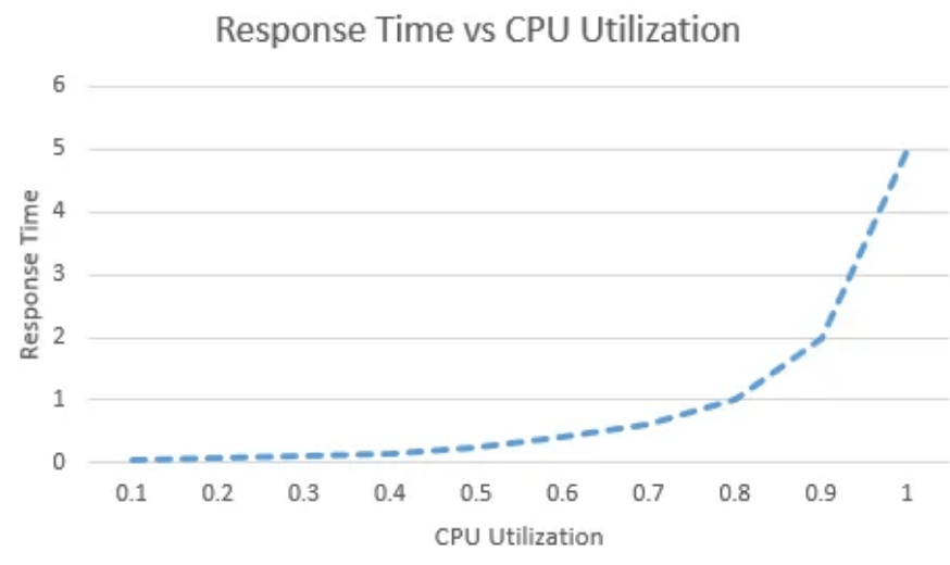
As shown, queuing time rises sharply when CPU utilization exceeds 70%. This threshold—often called the ‘knee’ of the hockey-stick curve—marks the point where delays become significant. Above this 70% mark, response times deteriorate quickly, underscoring how heavily utilization affects system performance.
This is the end of Part 1/4. Stay tuned for more.


Leave a reply to How to Assess CPU Stress (Part 3/4): CPU Run Queue Size – Yuan Yao, An Oracle ACE’s Blog Cancel reply