Yuan Yao, An Oracle ACE's Blog

The database CPU is already running at 100% utilization. You might expect adding more work to the database to make the system slower. Yet, as this example shows, the system can become faster. Let’s look at a demonstration.

1. SQL Driven by Java: When Database CPU Becomes the Bottleneck

Let’s begin with the host CPU view. The AWR report shows a system under severe CPU pressure: host CPU utilization is close to 100%, and the ending load average is 496.89.

Figure 1. AWR Host CPU.

The test used SwingBench SOE with 500 concurrent sessions running Browse Products for about seven minutes, with zero think time.

Here are the database’s top foreground events:

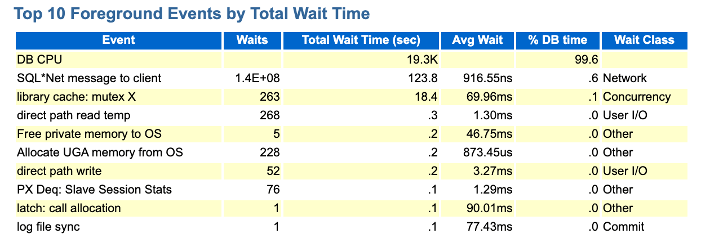
Figure 2. AWR Top 10 Foreground Events.

DB CPU accounts for 99.6% of DB Time. This means the workload in this demonstration is almost entirely CPU-bound.

The database CPU is clearly the application’s bottleneck. The obvious response would be to reduce CPU pressure. But what happens if we move the business logic into the database and ask that already-busy CPU to do even more?

2. The PL/SQL Version Delivers Much Higher Performance

SwingBench offers two implementations of the same workload. The first is the SQL version, shown in the previous section’s AWR reports. Java sends SQL statements to the database one at a time through JDBC. The application handles the business logic, while the database applies the data changes. In the second implementation, the PL/SQL version, Java calls a stored procedure through JDBC. The database then handles both the business logic and the data changes.

The results below come from the same environment: 500 concurrent users running Browse Products for seven minutes.

Metric	SQL version	PL/SQL version
TPS	33.4k	64.4k
Average latency	14.91 ms	3.05 ms

The PL/SQL version nearly doubles throughput. Average latency falls from 14.91 ms to 3.05 ms, a reduction of about 80%.

The puzzling part is this: if the CPU is already saturated processing data changes, how can the system become more efficient when the CPU handles both the business logic and the data changes?

3. Why Is the PL/SQL Version So Much Faster?

We’ll start with the Load Profile to estimate SQL executions and client calls per transaction, then look at CPU usage, Time Model Statistics, network communication, and thread context switching.

3.1 Load Profile Comparison

The SQL version is on the left and the PL/SQL version is on the right:

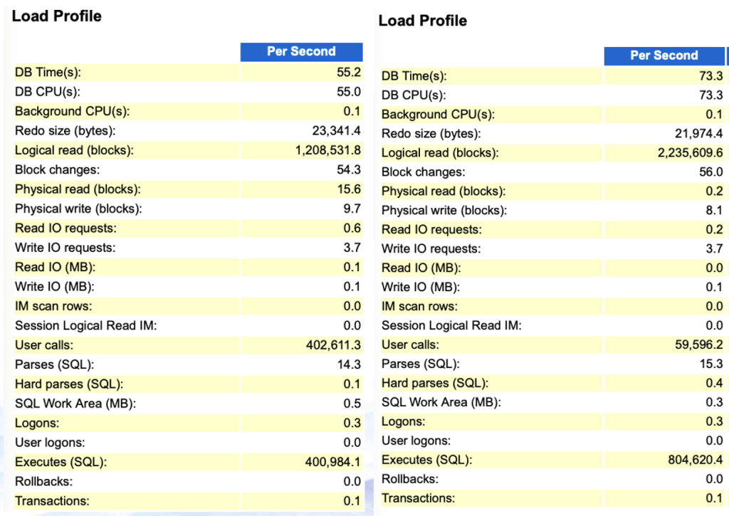
Using SwingBench TPS and the AWR Load Profile, we can estimate the number of SQL statements executed and database calls made per transaction.

Metric	SQL version	PL/SQL version
TPS	~33.4k	~64.4k
User calls/s	402,611	59,596
SQL executions/s	400,984	804,620
SQL executions per user call	~1	~13
SQL executions per transaction	~12	~12
User calls per transaction	~12	~1

For one Browse Products transaction:

• The SQL version makes about 12 User calls and executes about 12 SQL statements.
• The PL/SQL version makes about 1 User call and still executes about 12 SQL statements.

3.2 CPU Comparison

First, let’s look at CPU utilization in the PL/SQL version:

Both versions use nearly 100% of CPU, but two measures differ substantially:

1. The share of CPU used by %system falls from 25.7% to 5.3%.
2. Load average falls from 497 to 160.

3.3 Time Model Statistics

The combined image compares the two AWR Time Model Statistics reports: the SQL version is on the left and the PL/SQL version is on the right.

The sql execute elapsed time accounts for 49.5% of DB Time in the SQL version and 94.2% in the PL/SQL version.

Although database CPU is close to fully utilized in both cases, the share of DB Time spent executing SQL is very different. In the SQL version, a much larger share of DB Time is spent in the call path, including session switching, SQL*Net processing, and transitions into and out of the kernel.

3.4 How Much Does Network Communication Matter?

Each transaction in the SQL version requires 12 communications between the application and the database. That may suggest network communication has a large effect on transaction time. How large is it in this test? Let’s compare the Top 10 Foreground Events from both AWR reports.

SQL version

Event	Waits	Total wait time (sec)	Average wait	% DB Time	Wait class
DB CPU	—	19.3K	—	99.6	—
SQL*Net message to client	1.4E+08	123.8	916.55 ns	0.6	Network

PL/SQL version

Event	Waits	Total wait time (sec)	Average wait	% DB Time	Wait class
DB CPU	—	22.7K	—	100.0	—
SQL*Net message to client	18,406,596	20.8	1.13 μs	0.1	Network

In the SQL version, the average wait for one SQL*Net message to client is 916.55 ns. Based on the calculation in section 3.1, one Browse Products transaction makes about 12 client calls:

916.55 ns × 12 = 10,998.6 ns ≈ 11 μs ≈ 0.011 ms

In the PL/SQL version, the average wait associated with one call is:

1.13 μs × 1 ≈ 1.13 μs

The difference is about 10 μs, or 0.01 ms. That alone cannot explain the roughly 11.86 ms gap between the SQL version’s 14.91 ms average latency and the PL/SQL version’s 3.05 ms.

3.5 How Costly Is Thread Context Switching?

The main source of the performance gap is that the PL/SQL version moves business logic from the application into the database. Multiple SQL calls are wrapped in a single PL/SQL call, substantially reducing process context switching (thread context switching).

The CPU breakdown provides supporting evidence. In the SQL version, %system accounts for 25.7% of CPU time, compared with only 5.3% in the PL/SQL version. %system represents time spent in the operating system kernel, including scheduling, context management, and other housekeeping work. The much higher value in the SQL version is consistent with more frequent context switches and their associated overhead. The higher call rate points in the same direction: the SQL version makes about 12 user calls per transaction, compared with about 1 in the PL/SQL version. Each call crosses the application–database boundary and creates another opportunity for process and thread switching.

Everyone knows that context switching is expensive, but most people underestimate just how expensive it can be. The following widely circulated chart gives approximate orders of magnitude for different computer operations:

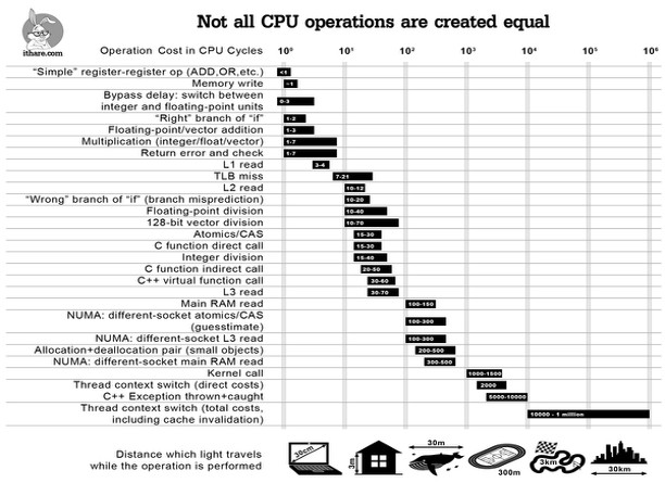
The figures shown are estimates:

• Direct C function call: 15–30 cycles
• Indirect C function call: 20–50 cycles
• Main memory read: 100–150 cycles
• Thread context switch, direct cost: about 2,000 cycles
• Thread context switch, total cost including cache disruption: 10,000–1,000,000 cycles

At 2 GHz, 1,000,000 cycles take about 0.5 ms.

It is like trying to work while being interrupted: after switching to another task, it takes time to regain your train of thought. The issue is not only how fast each piece of work is, but how often execution is interrupted and has to switch context.

4. Takeaways

• A CPU core can execute one thread at a time. The operating system uses time-slicing to let multiple processes and threads take turns.
• Context switching has indirect costs, including scheduling, saving and restoring state, and loss of cache locality.
• As CPU utilization approaches saturation and runnable threads grow, competition and queuing increase. Involuntary context switches can become more frequent, making switching and scheduling costs more visible in throughput and latency.
• Efficient CPU use often means reducing unnecessary switches and letting each call complete a meaningful batch of work.
• This principle applies to any processes and threads scheduled by an operating system. Databases are one example; the same concerns apply to Oracle, MySQL, PostgreSQL, application processes, and background processes.
• If frequent database calls are slowing an application, a full rewrite is often unnecessary. Start with the small number of hot transactions that make the most calls or execute most often. Batch SQL (for example, JDBC addBatch/executeBatch), set-based SQL, or stored procedures can reduce call volume. These hot paths may represent only a small share of the application’s code or transaction types—perhaps 10%—yet account for most database calls and CPU overhead.